Get Rich or Buy Trying - Part 2 [Solution]

Solution for the week of 10/13/24

Our problem from 10/6/24 was

Consider the following stock behavior:

1. The stock’s value will change by a factor of (1+δ) from it’s pervious value each minute where δ is uniformly distributed from [-1/1000, 1/1000]. For example after two minutes, the value would be p_0 * δ_1 * δ_2.

Your job is to determine the distribution of the value of the stock after 1 day. Assume the stock is traded for 7 hours a day (a bit off, I know).

Unfortunately we didn’t get any responses this week—perhaps because it was a bit of a tricky problem. On that note, I’d like to encourage folks to submit partial solutions even just thoughts on how to solve the problem. For some of these more challenging problems, I’m always curious if people find simpler or just different ways of solving :)

Now concerning the problem, I had to do a bit of digging myself to figure out how to go about this problem. My full solution is posted here. My first thought was to transform the problem into log space

\(Y = X_1 \cdot X_2 \cdot \ldots \cdot X_{420}\)

where X_i is a random variable that is uniformly distributed from [.999, 1.001]

\(\displaystyle Y = \prod_{i=1}^{420} X_i \rightarrow \ln(Y) = \sum_{i=1}^{420} \ln(X_i)\)

My next though was then to do repeated convolutions over these new random variables ln(X_i). It became clear quite quickly that this was going to be difficult (even with software) so instead, I dug a round a little bit more and stumbled on using characteristic functions, which allow for simpler algebra over random variables once they’ve been transformed to their Fourier dual. The challenge emerged at the end when I had to perform the inverse transform over the product of characteristic functions.

\(\displaystyle f_{Y}(y) = \frac{1}{2\pi} \int_{-\infty}^{\infty} e^{it \ln(y)} \left( \frac{b^{1-it} - a^{1-it}}{(b-a)(1-it)} \right)^{420} \, dt\)

This integral seemed rather intimidating so I poked around for another method. I found a slightly different approach in Springer’s Algebra of Random Variables. This slightly different method uses what’s known as the Mellin transform.

\({\displaystyle \left\{{\mathcal {M}}f\right\}(s)=\varphi (s)=\int _{0}^{\infty }x^{s-1}f(x)\,dx}\)

After performing roughly the same steps, you end up with the following integral.

\(\displaystyle \frac{1}{2\pi i} \int_{c-i\infty}^{c+i\infty} x^{-s} \left( \frac{b^s - a^s}{s(b-a)} \right)^{420} \, ds\)

Computing this integral requires the Residual Theorem which results in computing the following derivative

\(\displaystyle \text{Res}(f, 0) = \frac{1}{419!} \left( \frac{1}{b-a} \right)^{420} \lim_{s \to 0} \frac{d^{419}}{ds^{419}} \left( \frac{(b^s - a^s)^{420}}{x^s} \right)\)

This felt a bit easier so we went down this route and got the following final analytic expression.

\(\displaystyle f_{Y}(y) = \frac{1}{419!} \left( \frac{1}{b-a} \right)^{420} \sum_{k=0}^{420} \binom{420}{k} (-1)^k c_k^{419} \cdot \mathbb{1}_{c_k > 0}\)

where

\(c_k = k \ln(b) + (420-k) \ln(a) - \ln(y) \text{ and } b=1.001, a=.999\)

As it turns out, computing the value of this distribution runs into numerical stability issues. Despite attempting various tricks for improving numerical stability including converting the computation into log space and allowing for high precision floating point number, I couldn’t get the computations of this exact solution working well so I could verify it against empirical results. To do that, I reverted back to my characteristic function approach and used a Fast Fourier Transform to approximate the distribution. With this, I was able to verify that the approximate, exact, and empirical distribution all matched for more numerically stable parameters giving me confidence that the solution above is correct and the exact solution. Though, this problem make very clear that exact solution aren’t very useful if they can’t be realistically computed.

Below is a plot of the distribution.

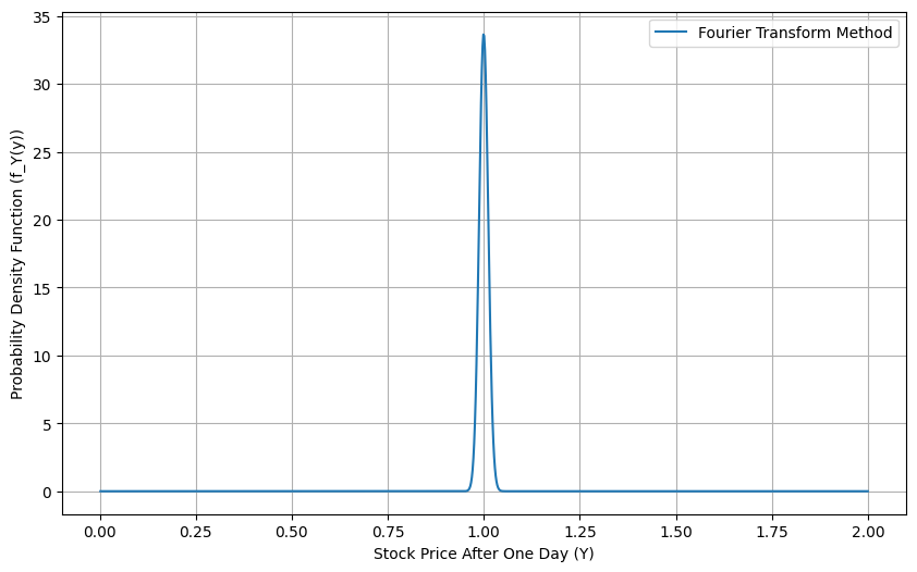
As Sal Elder pointed out last week, this distribution is approximately log-normal. The log comes from the fact that we’re multiplying our random variables (see the first equation) and the normal part comes from the rather large sample size of 420 in this problem.

I hope you found this problem fun! As always, feel free to leave comments, thoughts, etc. in the comments. Also, feel free to DM with any ideas you have for a puzzle! Hope to see you for the next one!